ODEAction

Figure 1: action generation paradigms, water-filled cup execution, end-effector trajectories, and representative results — **Figure 1. From action-chunk prediction to continuous action evolution.** (a) Base Policy uses action-chunk prediction and is prone to abrupt action changes at chunk transitions, whereas ODEAction's continuous evolution ensures that action trajectories are generated continuously. Comparisons of real-robot task execution and the corresponding end-effector trajectories illustrate the differences in execution smoothness and trajectory continuity between the two methods. (b) Representative results on EBench simulation and real-robot tasks: compared with Base Policy, ODEAction increases the task success rate (SR) and reduces the end-effector mean absolute jerk (EE-MAJ).

01 Idea

From action chunks to action evolution.

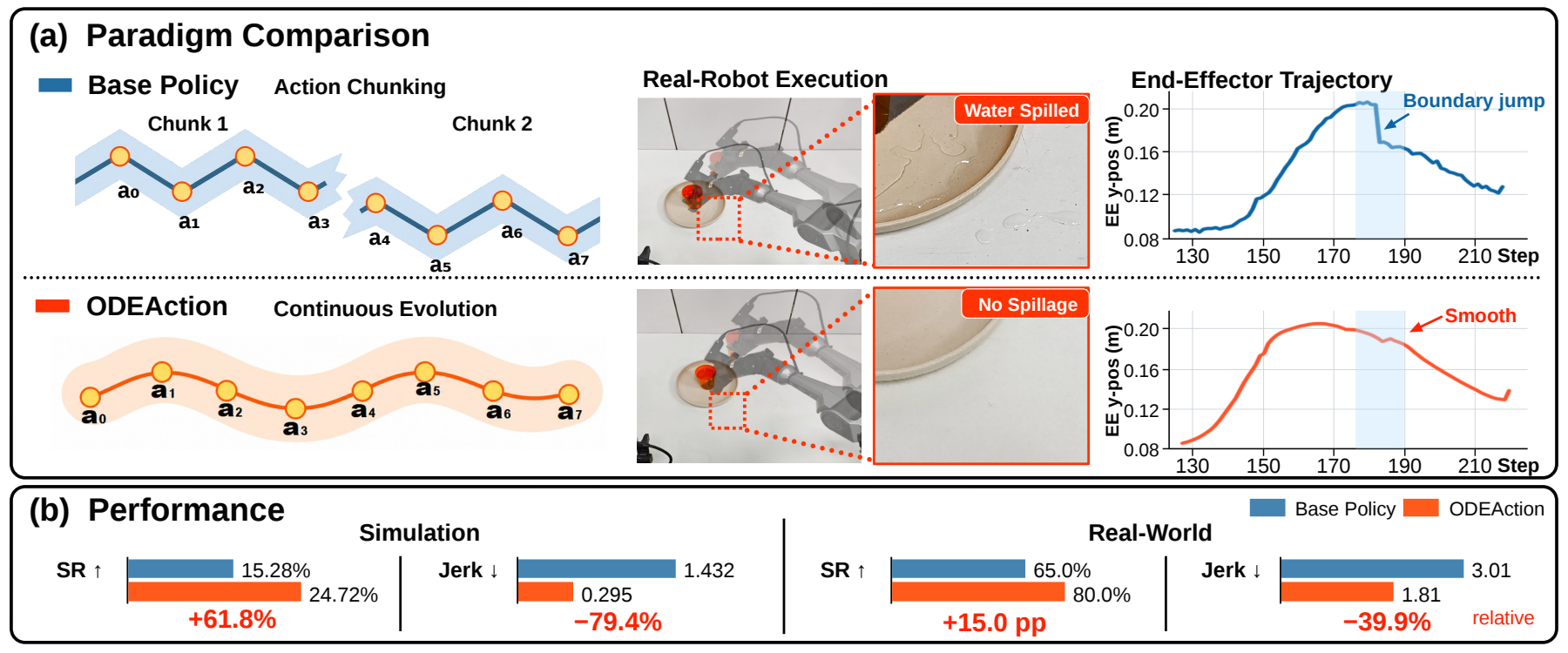
Vision-language-action models typically predict a sequence of future actions as an action chunk. The robot executes these actions, then switches to a newly predicted chunk. Switching between separately predicted chunks can introduce abrupt changes at their boundaries.

ODEAction changes the prediction target: it learns the evolution rate of the current action. Starting from that action, integrating its learned evolution rate generates subsequent actions, each connected to the one before it. This is the shift from predicting future action chunks to Continuous Action Evolution.

How does action generation shape execution?

A real-robot experiment illustrates the difference between the two action-generation paradigms. The robot must move a water-filled cup smoothly onto a plate without spilling. In Figure 1(a), the execution images and end-effector trajectories show the contrast: a trajectory jump accompanies a spill under the action-chunking policy, while ODEAction completes the motion with a smoother trajectory and no spillage.

This brings us to the next question: how can demonstrations teach continuous action evolution?

02 Method

Learn an action transition field.

We describe continuous action evolution with an ordinary differential equation (ODE), and define its vector field as the Action Transition Field. Given a query action, evolution time, and task conditioning, this field specifies the action's evolution rate.

Figure 2 connects three steps: construct a target field from demonstrations and their neighborhoods (a), learn the conditional field through direct supervision (b), then integrate the learned field from the current action during inference (c). Together, these steps turn demonstrated actions into a model of how actions evolve.

Figure 2. Learning the action transition field and recursively generating actions. (a) Discrete demonstrated actions are interpolated into a continuous trajectory. Target transition vectors are constructed by combining progression along the demonstration with deviation correction, inducing a target action transition field F* in the trajectory neighborhood. (b) During training, the action transition field (Fθ) is learned through direct supervision. (c) During inference, the current action serves as the initial condition, and subsequent actions are recursively generated by numerically integrating the learned action transition field using an ODE.

Build the target evolution rate from demonstrations.

First, interpolation connects discrete demonstrated actions into a continuous path γ(τ). Its tangent describes the direction and rate of demonstrated progression. Recursive generation can drift away from this path, so we also sample nearby actions, extending supervision into its neighborhood.

At each query action, the progression component follows the demonstration at the corresponding evolution time. The correction component points toward the corresponding demonstrated action. Their sum gives the target evolution rate. The animation below explores how these components change along and around the path; switch to manual exploration to choose your own query.

An action, two components, one direction

Target Action Transition Field · F*

Vector composition

ProgressionCorrectionTarget direction

Along the demonstrationDeviation from the path

F*(a, τ) = γ̇(τ) + k (γ(τ) − a)Progression + correction

Learn the field through direct supervision.

The target field supplies an evolution rate for each sampled action and evolution time. Conditioned on the current observations and task instruction, the model learns to predict this vector. Training directly minimizes the difference between the predicted and target vectors, without solving an ODE.

This is the field-learning step in Figure 2(b): demonstrations and nearby query actions teach the model how actions evolve, both on and around the demonstrated path.

Generate actions through recursive integration.

At inference, the learned field drives action generation. We begin with the current action as the initial condition. Each integration step queries the field for an evolution rate and uses it to produce the next action. That action becomes the starting point for the following step, creating explicit dependencies throughout the generated sequence.

Implemented as a modular action head, ODEAction can bring this generation paradigm to different vision-language backbones. The experiments examine whether this change improves both task completion and the quality of motion.

Recursive action evolution

aₙ₊₁ = aₙ + Δτ Fθ(aₙ, τₙ | c)

Learned Action Transition Field · Fθ

Evolution time0 / 40

Query the field → update the action → continue from the new action.

03 Experiments

We evaluate both what the robot completes and how it moves. Success rate measures task completion; four complementary trajectory metrics describe motion smoothness and continuity.

We begin with LIBERO and EBench, then examine the relationship between boundary continuity and task success. We next test a different backbone on RoboTwin, compare with action-chunk continuation methods, and evaluate real-robot performance. Ablation experiments then examine the roles of neighborhood supervision and correction.

Comparison with action chunking

Using π₀.₅ as the base policy, we compare the two generation paradigms on LIBERO and EBench. These benchmarks connect task-level outcomes with the smoothness and continuity of the generated actions.

Boundary continuity and task success

The improvements above lead to a further question: how does improved boundary continuity relate to task success? Figure 3 pairs the reduction in boundary discontinuity with the gain in success rate for each evaluation unit.

We find a consistent pattern: larger reductions in boundary discontinuity tend to accompany larger gains in task success, with a strong positive correlation. This connects improvements in generated motion with improvements in task execution.

Figure 3. Relationship between improvements in boundary continuity and gains in task performance. (a) Four LIBERO suites and six EBench tasks arranged in descending order of Boundary Discontinuity Reduction (BDR). (b) Success-rate gains (SR gain) of ODEAction relative to Base Policy, shown in the same evaluation-unit order. BDR and success-rate gains exhibit a strong positive correlation across the ten evaluation units.

Generality of the generation paradigm

Can the same generation paradigm work with another vision-language backbone? We integrate ODEAction with StarVLA-OFT and evaluate it on RoboTwin. Its modular action head brings continuous action evolution to a different backbone and bimanual task setting.

Comparison with action-chunk continuation methods

We next compare with methods that improve continuity within chunk-based action generation. This comparison examines how learning action evolution performs alongside approaches that improve connections between action chunks.

ODEAction achieves the best average success rate and all four trajectory-quality scores, improving task completion and motion quality together.

Real-robot experiments

The gains carry over to real robots. On the AgileX Cobot Magic platform, we evaluate tasks spanning pick-and-place, opening a drawer, carrying a water-filled cup, and inserting a spoon.

Average success rises from 65% to 80%, and all four trajectory-quality metrics improve. The task images and results below show how continuous action evolution translates into physical execution.

Ablation experiments

We use ablation experiments to examine the effectiveness of neighborhood supervision and correction. Without neighborhood supervision, generation becomes less robust: actions can leave the region where evolution directions were learned. Without correction, evolution can continue, but deviations remain uncorrected.

Without neighborhood

Supervision follows the demonstrated path.

Without correction

Progression continues; the offset remains.

Progression and correction recover the path.

How neighborhood supervision and correction shape action evolution.

Together, neighborhood supervision and correction support robust action evolution. The full ODEAction also achieves the highest task success in the ablation experiments.

Table 4 · Ablation experiments

Task success (%) ↑

From predicting chunks to evolving actions.

By learning how actions evolve and generating them recursively, ODEAction changes the basis of action generation. Across simulation benchmarks and real robots, this paradigm improves both task performance and trajectory quality.

Explore the full paper ↗

Cite this work